Tutorial 10 - DG and AMR

In this tutorial, we solve the Poisson equation using a discontinuous Galerkin discretization and adaptive mesh refinement.

The setup is taken from Elman, H. C., Silvester, D. J., & Wathen, A. J. (2014). Finite elements and fast iterative solvers: with applications in incompressible fluid dynamics. It is a standard test case that introduces a singularity at the origin. Due to this singularity, regular global refinement does not meet the expected optimal a priori error estimates. This issue is in practice usually circumvented by adaptive local refinement around the singularity.

The analytical solution to the Poisson equation

\[ \begin{eqnarray*} - \Delta u = f \end{eqnarray*} \]

is given in polar coordinates by

\[ \begin{align*} u(r, \theta) &= r^{2/3} \sin( (2 \theta + \pi) / 3 ), \\ f &= 0. \end{align*} \]

This tutorial demonstrates how adaptive mesh refinement (AMR) is applied together with the discontinuous Galerkin method. For details on the discretization we refer to the literature, for example Rivière, B. (2008). Discontinuous Galerkin methods for solving elliptic and parabolic equations: theory and implementation.

Domain setup and refinement.

We first create the PrimitiveStorage from a mesh file has has been done in previous examples.

Mesh refinement procedures can be split into two types.

• Conforming algorithms refine the mesh while keeping a conforming structure. That means, no hanging nodes are created. This has the advantage that standard conforming finite element discretization can still be applied without any modification. The disadvantage of this method is that it might produce ill-shaped elements.
• Non-conforming algorithms may maintain the quality of the elements. However, in general those methods may produce hanging nodes and the standard conforming finite element discretizations cannot be applied directly. Non-conforming discretizations, on the other hand can still be applied.

In this tutorial we cover the second case - and thus apply a discontinuous Galerkin discretization to the problem. However, the first method is also applicable in HyTeG.

The refinement is applied directly to the PrimitiveStorage and yields a tree-like structure. When a (volume-)primitive is refined, child primitives are created. In 2D, faces are split into 4 face primitives, in 3D cells are split into 8 cell primitives. This works as described in Bey, J. (1995). Tetrahedral grid refinement.

The algorithm, however, is restricted to maintain a 2:1 balance between neighboring volume primitives. That means the refinement levels of neighboring macros can only differ by 1. Before the refinement is applied, the marked primitives are passed to a function that marks further primitives for refinement if necessary to keep the 2:1 balance.

All of this happens in one method. It requires only to pass the PrimitiveID of all (local) volume primitives to be refined.

   // Refining multiple times at the boundary.
   for ( uint_t i = 1; i <= refinementsAtOrigin; i++ )
   {
      // Here we collect all face IDs of faces that we want to refine.
      std::vector< PrimitiveID > facesToRefine;
 
      auto faceIDs = storage->getFaceIDs();
 
      // Looping over all macro-faces.
      for ( auto faceID : faceIDs )
      {
         auto face              = storage->getFace( faceID );
         auto vertexCoordinates = face->getCoordinates();
 
         real_t eps      = 1e-8;
         auto   atOrigin = [eps]( const Point3D& x ) { return x.norm() < eps; };
 
         // If any vertex of the face is near the origin, mark for refinement.
         if ( std::any_of( vertexCoordinates.begin(), vertexCoordinates.end(), atOrigin ) )
         {
            facesToRefine.push_back( faceID );
         }
      }
 
      // Eventually we start the refinement process. Note that possibly additional macro-faces are refined to maintain the 2:1
      // balance.
      storage->refinementHanging( facesToRefine );
   }

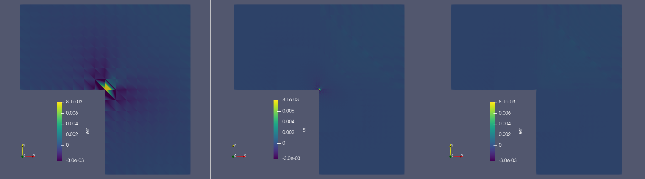
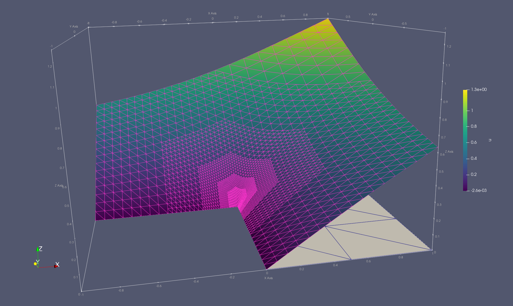
In this example we simply refine all primitives that have a vertex at the origin multiple times. The result looks like this:

initial coarse grid

after 2 refinements

after 5 refinements

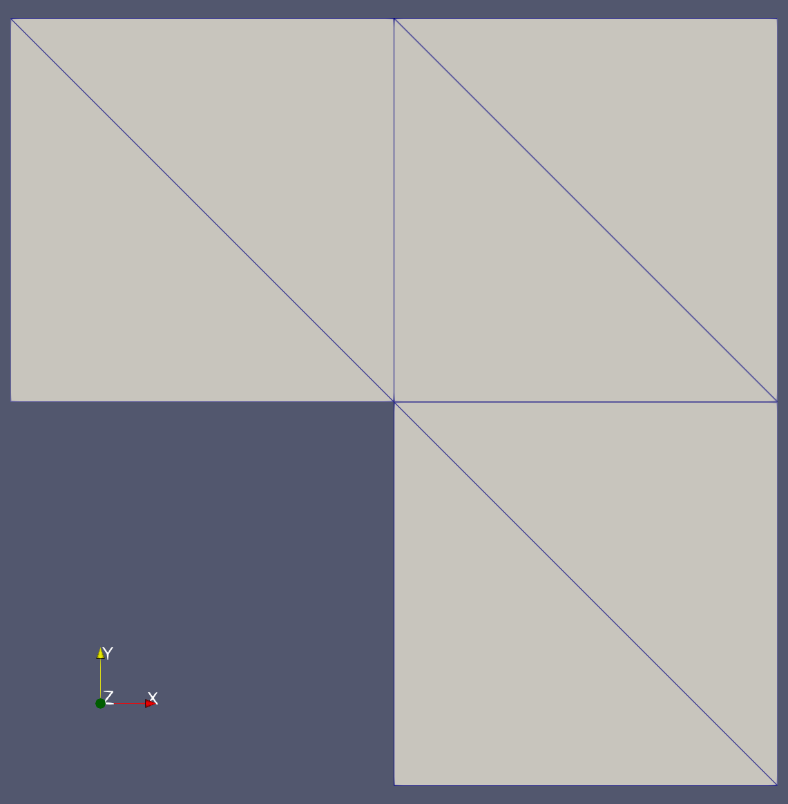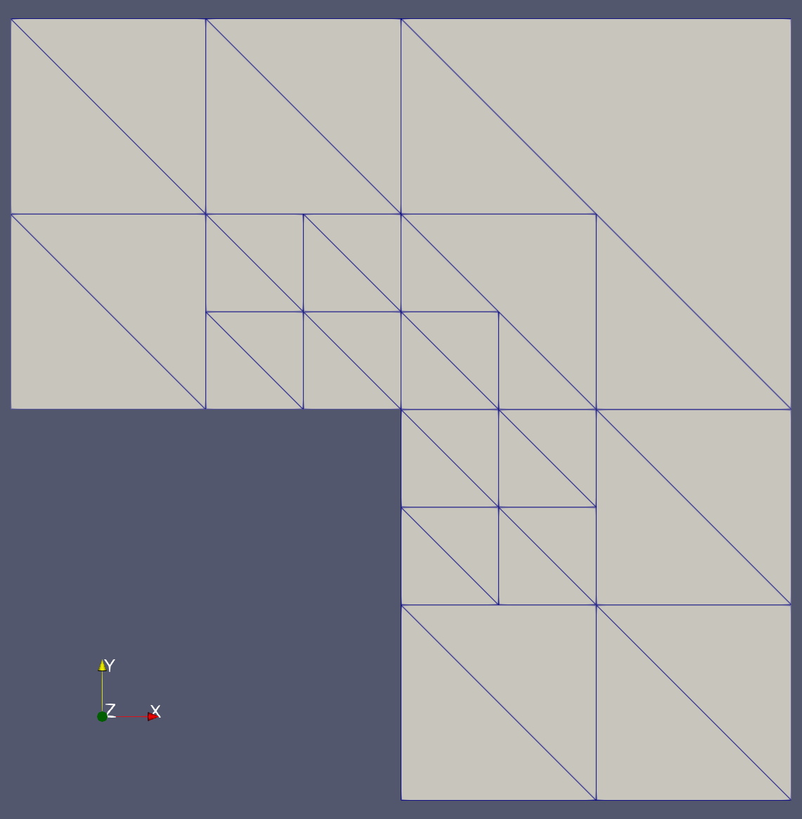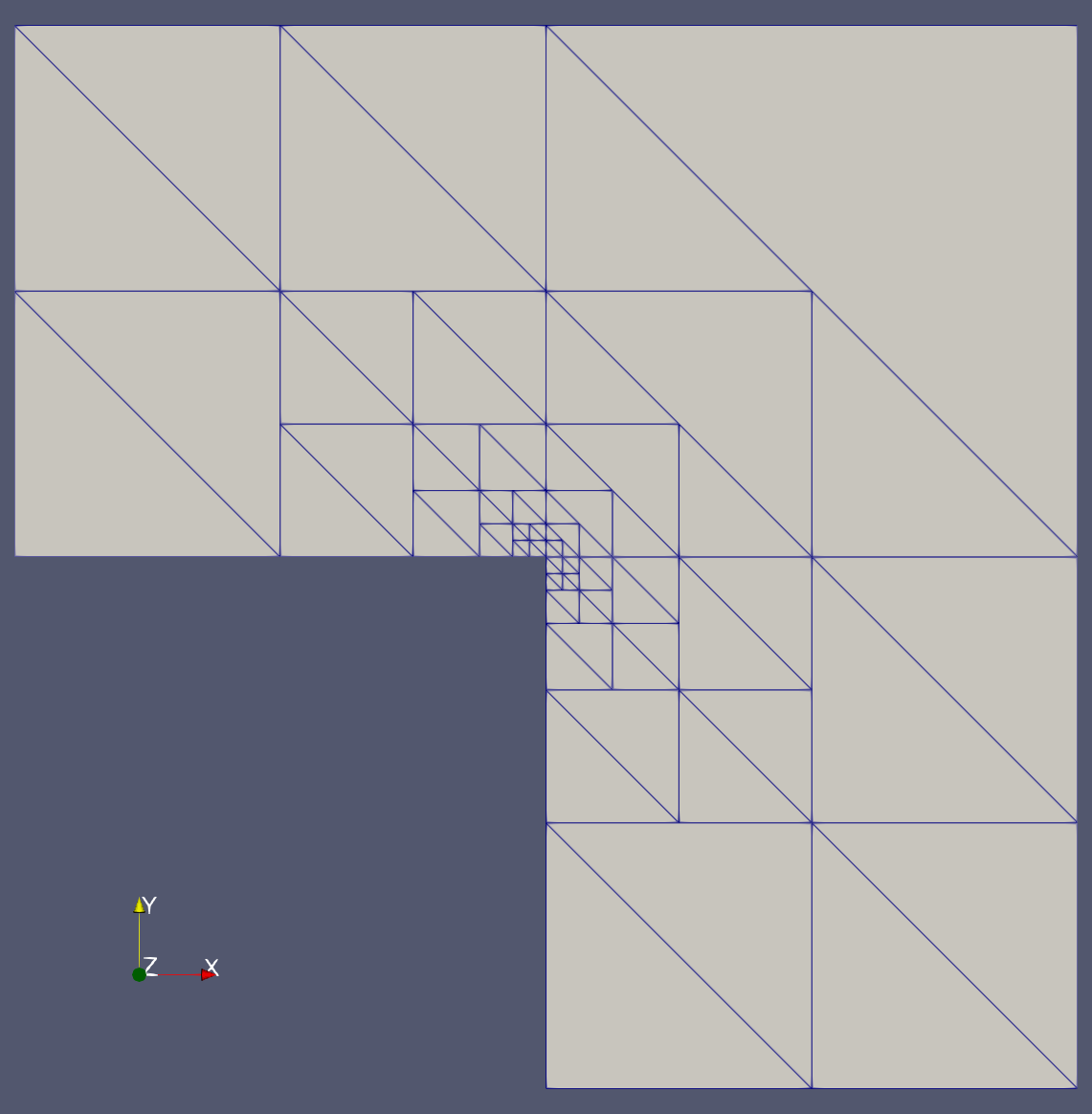In a second step, these coarse grids are refined uniformly.

Discontinuous Galerkin

DG functions and operators are almost used as it's done for other conforming discretizations. The main difference is that the basis and degree are passed in the constructor. This also applied for the operators - the form has to be passed here, too.

   auto basis       = std::make_shared< DGBasisLinearLagrange_Example >();
   auto laplaceForm = std::make_shared< DGDiffusionForm_Example >( 1, solution, solution );
   auto massForm    = std::make_shared< DGMassForm_Example >();

   DGFunction< real_t > u( "u", storage, globalMicroRefinements, globalMicroRefinements, basis, 1 );
   DGFunction< real_t > f( "f", storage, globalMicroRefinements, globalMicroRefinements, basis, 1 );

   DGOperator A( storage, globalMicroRefinements, globalMicroRefinements, laplaceForm );
   DGOperator M( storage, globalMicroRefinements, globalMicroRefinements, massForm );

The weak enforcement of Dirichlet boundary conditions is handled by a function that also takes as an argument the Form object.

Interpolation of functions into the finite element space is currently handled by solution of the system

\[ \begin{eqnarray*} M u = (f, v)_\Omega \end{eqnarray*} \]

That requires the solution of a linear system involving the mass matrix \( M \):

   tmp.evaluateLinearFunctional( solution, globalMicroRefinements );
 
   PETScCGSolver< DGOperator > solverM( storage, globalMicroRefinements, numerator );
 
   solverM.solve( M, sol, tmp, globalMicroRefinements );

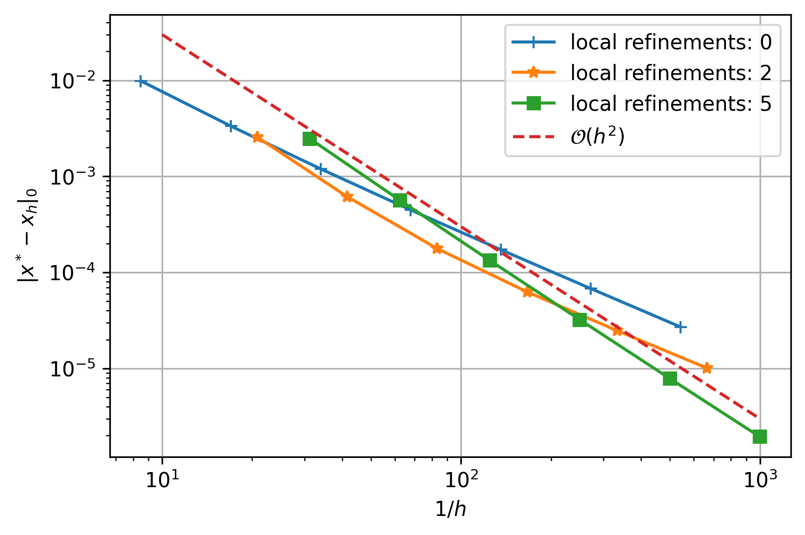
Eventually, we solve the linear system and plot the error over \( \frac{1}{h} \).

   PETScCGSolver< DGOperator > solverA( storage, globalMicroRefinements, numerator, 1e-12, 1e-12, 10000 );
   solverA.solve( A, u, f, globalMicroRefinements );

   err.assign( { 1.0, -1.0 }, { u, sol }, globalMicroRefinements );
 
   M.apply( err, Merr, globalMicroRefinements, All, Replace );
   auto discrL2 = sqrt( err.dotGlobal( Merr, globalMicroRefinements, Inner ) );

error vs refinement

error vs DoFs

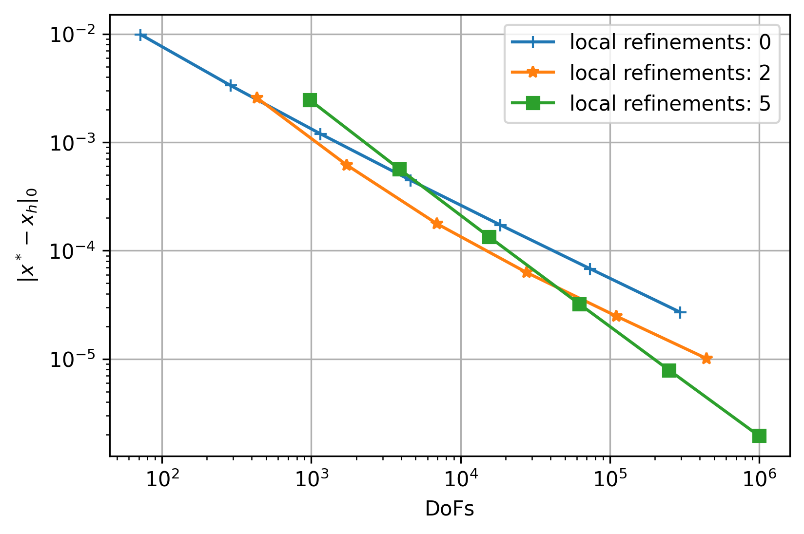Standard global refinement is not sufficient to retain the optimal asymptotic accuracy. But with aggressive local refinement the accuracy can be recovered.

Plot of the error on different macro-refinement levels (0, 2, and 5). Uniform level is 3 for all three images.

Plot of the computed solution and the mesh after 5 local and 3 uniform refinement steps.